So how much does OpenAI owe us?

Introduction: Copyright Law and Whatnot

I recently watched a clip from a debate between Timothy Nguyen of Google Deepmind and Danish author Janne Teller. The debate, entitled Technology and Freedom, took place at Hay-on-Wye in summer 2025. On the subject of copyright, Nguyen says:

The reason AI is so powerful is because it’s scraped all this data on the internet and of course that has all these issues in terms of copyright law and whatnot. But that’s also democratised knowledge and so there are ways in which it’s been good and bad. But now we have this very intelligent system which has all this knowledge from books, but then maybe there are going to be some authors who aren’t going to be very happy. So there are always going to be winners and losers.

Teller replies:

This is an undermining of any intellectual property rights we have developed up to now. Anything you have written on a Facebook post which is public will be considered by this Metaverse as something they can use to develop their AI and you might say OK, that’s a new form of sharing. Anything you contribute, everybody owns it. But then that speaks to nationalising all technology platforms. You want to have everything everyone else has created. But then we want to have your work also and have control over it.

The clip cuts off here and I haven’t seen a video of the full debate, so I don’t know how Nguyen replied. But I think Teller made a good point. It’s not just that LLMs have been trained (illegally) on masses of copyrighted material. They have also been trained on data from the internet, which is a public good, and perhaps the people who unwittingly created all the training data should be entitled to some sort of compensation. Even the slopigarchs themselves acknowledge this. For example, in 2017, Elon Musk said that the pace of change is:

a massive social challenge. And I think ultimately we will have to have some kind of universal basic income (UBI). I don’t think we’re going to have a choice.

At the moment we are facing two possible outcomes. Either AI progress grinds to a halt and the bubble bursts, or AI breakthroughs continue to happen at a rapid pace, replacing human jobs, and everyone ends up becoming unemployed until they can find other jobs to do. Every previous improvement in technology, no matter how disruptive, eventually ended up with people finding other things to do, so the economy will keep going somehow. But before we reach that point we may find ourselves facing serious social unrest. As Teller suggests, perhaps it is the AI companies themselves who should pay for this. After all, they did steal everyone else’s work to train their models. But if, in some grim future in which companies like OpenAI become profitable, we eventally get compensation, how much compensation should we get?

It seems like this question has no answer. But actually there’s a simple heuristic for evaluating the relative contributions of the model and the data, which I want to explain in this post. Not only is this heuristic relevant for musing about the future of AI, but it’s also surprisingly useful in everyday data science, too.

The Cover-Hart Theorem

Consider a classification problem in which the input is a data point $x$ contained in some metric space (i.e. a set equipped with a notion of distance) $(X, d)$, and the output is a classification into one of $M$ classes. The classifier is evaluated by the percentage of data points which it classifies correctly (the accuracy). If $A$ is the accuracy then $R = 1-A$ is called the error rate.

The Bayes Rate $R^\ast$ for the problem is defined to be the best possible accuracy which any classifier could have. Why isn’t $R^\ast$ just 100%? That’s because the same point might appear in more than one class! See the example below.

Suppose a data set $\mathcal{X}$ is given. It consists of some points $x_i \in X$ and the corresponding classes $\theta_i$. We want to use the data set $\mathcal{X}$ to build a classifier.

The 1-Nearest Neighbour or 1-NN classifier is the classifier $C$ which simply assigns an unseen data point $x$ to the class of the closest point to $x$ in $\mathcal{X}$ (for simplicity, let’s assume that $\mathcal{X}$ doesn’t contain any duplicate points). That is, if $d(x, x_i) = \min_{y \in \mathcal{X}}d(x, y)$ then $C(x) := \theta_i$. Note that to define the 1-NN classifier, we need $X$ to be a metric space, or else there is no notion of the nearest neighbour.

The theorem which Cover and Hart proved in 1967 is that the error rate $R$ of the 1-NN classifier satisfies

asymptotically as the number of data points in $\mathcal{X}$ goes to $\infty$, and provided that the points in $\mathcal{X}$ are an iid sample from some distribution.

In other words, if you are given a data set and asked to build a predictive model, just doing the most naive thing possible and looking up the closest point in your data set to the point you want to classify already gets you halfway to the lowest possible error.

Example

Here is an example which I used to use when teaching this topic in university courses.

Let’s consider a single predictor $x$. There are two classes labelled $0$ and $1$. The distribution of $x$ for class $1$ is $N(1, 1)$ and the distribution of $x$ for class $0$ is $N(-1, 1)$. Suppose the population is equally distributed among the two classes.

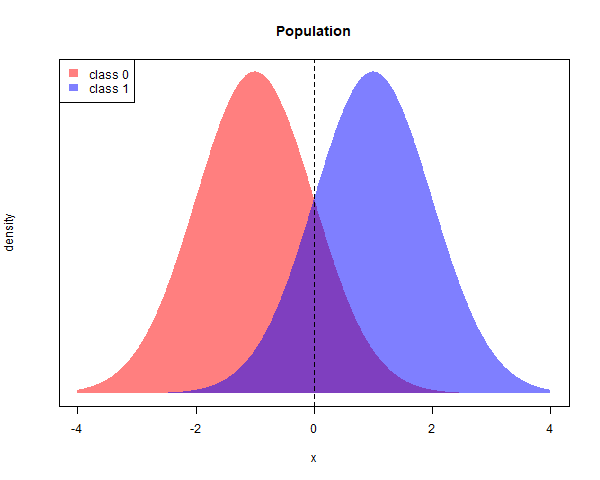
The best possible classifier would classify a point $x$ into whichever class has the higher density for that particular value of $x$. The purple area represents the proprtion of points which would be misclassified. Since 50% of the population is in each class, the purple area is equal to

bayes_rate <- 1-pnorm(1)
# 0.1586553

Now suppose we are supplied with a training dataset consisting of 50 points from each class

set.seed(100)

N <- 100
df_train <- data.frame(x = c(rnorm(N/2, 1, 1), rnorm(N/2, -1, 1)), y = rep(c(1, 0), each=N/2))

The following function classifies a point using the nearest neighbour with the metric being $d(x, y) = \lvert x-y \rvert$.

classify_point <- function(x, df){
  df$y[which.min(abs(x-df$x))]
}

To see whether the Cover-Hart Theorem works in this example, let’s create a test data set of 1000 new points.

M <- 1000
df_test <- data.frame(x = c(rnorm(M, 1, 1), rnorm(M, -1, 1)), y = c(rep(1, M), rep(0, M)))

The error rate of the 1-NN classifier on this data set can be calculated as follows

pred <- sapply(as.list(df_test$x), function(x) classify_point(x, df_train))
1 - sum(pred == df_test$y)/length(pred)
# 0.216

As expected, $0.216$ lies between the Bayes rate and twice the Bayes rate.

Of course, many other classifiers will perform better. For example, logistic regression already almost achieves perfect accuracy.

model <- glm(y~x, data=df_train, family="binomial")
pred_logistic <- round(predict(model, df_test, type="response"))
1 - sum(pred_logistic == df_test$y)/length(pred)
# 0.16

If you run the whole script again with the same seed but with N=10000 points in the training data, you will even find that logistic regression gets an error rate which is lower than the Bayes rate! This happens because the training and test sets are finite samples from the actual data distribution, so there is some sampling error.

Practical Use

There are two ways to use this in practice. First, suppose that you are presented with a data set and build a quick and dirty classifier using 1-NN and achieve an accuracy of 80%. Then the error rate $R$ of the 1-NN classifier is 20% and the Cover-Hart Theorem tells you that the Bayes rate $R^\ast \ge R/2$, so the Bayes rate cannot be less than 10%, which means that you can’t expect to achieve an accuracy of better than 90% using some other algorithm. This might be a helpful guide to how much time you should spend trying to build a better classifier. In practice, the quick and dirty classifier you build will be something other than 1-NN¹, and it usually has better performance than 1-NN, so this can actually be a useful way to estimate the Bayes rate on a new data set.

Secondly, suppose that you are presented with a classification algorithm with an accuracy of 95%. Then you can estimate that the Bayes rate $R^\ast$ is at most 5%, because $R^\ast$ is the lowest possible error rate among all classifiers. This means that the error rate of a 1-NN classifier $R$ cannot be more than 10%. But that means that a 1-NN classifier would have given you 90% accuracy. Since the 1-NN classifier is just another name for “look at the data”, you could already achieve 90% accuracy by looking at the data alone without building your fancy model. In other words, the data is doing $90/95 = 94.7\%$ of the work!²

Problems with the Cover-Hart Theorem

In practice, Cover-Hart should be used only as a heuristic and not as something which is expected to hold in all cases. This is because it makes very strong assumptions about the data.

• It’s only true if you have infinitely many data points, so it will only be approximately true in any real-life situation. How close the Cover-Hart Theorem is to being true in any real-life situation might also depend very strongly on the metric being used.
• More seriously, the data points need to be independent and identically distributed (iid). This is never true, despite the fact that textbooks and courses seem to suggest otherwise. In fact, I think it’s rare for training and test sets even to come from the same distribution.

For example, consider image classification. Cover-Hart suggests that you can classify any image correctly if you find the closest image, perhaps in the sense of Euclidean distance, in some sufficiently large reference data set. But clearly the reference data set would have to be massive, and the cost of searching for the closest image would probably be extremely high.

What does Cover-Hart say about AI?

The Cover-Hart Theorem, then, doesn’t suggest a sensible way to build an AI model. For example, suppose you want to generate the next word, given a string of text. A 1-NN classifier would be supplied with a corpus of data. It would need to search through this data and find the piece of text that was the closest match to the given string, and then extract the next word from that piece of text. For some kinds of text, like The capital of France is, this might work well, but clearly it’s not going to be a good approach in general.

This isn’t how Large Language Models work at all, so how is the Cover-Hart Theorem relevant to LLMs? Well, I think it could be used as a heuristic for measuring the relative contribution of the model and the data. For example, let’s suppose an LLM has an accuracy performance of $A$ percent on some benchmark. Then, as explained above, a 1-NN classifier could be expected to achieve an error rate of $2(1-A)$ and so you could estimate that the data by itself is contributing roughly

of the overall performance. This could be taken as a measure of how much the data is “worth” versus the model.

For example, if an AI company achieves 80% on some benchmark, then the people who contributed the data in some sense deserve $(2(0.8)-1)/0.8 = 75\%$ of the credit.

Who was right?

So was Teller correct? Do the people who generated the data deserve most of the profits (if there are any) from AI? Well, that depends on what you mean by “AI”.

In the case of LLMs, assuming that they really are able to replace people in the workplace, I think the Cover-Hart Theorem could provide a first step for deciding how to regulate or tax. But the term “AI” encompasses a lot of different models, and some of those models don’t use training data at all. For example, AlphaZero reached grandmaster-level performace in chess and superhuman performance in go by playing against itself. And this isn’t a new idea; in the 1990s TD-Gammon was already able to outperform humans in backgammon by taking a similar approach. Personally I find these kind of algorithms even more impressive than LLMs, but that’s just my opinion.

One more thing. Suppose we did find ourselves in a world in which a government was choosing to tax AI companies based on the above formula. Then we could reach a bizarre scenario in which, in order to avoid tax, the AI companies would be competing to make the ratio $(2A-1)/A$ as small as possible. This would mean that, instead of boasting about the accuracy of their models on self-chosen benchmarks, these firms would find themselves in a paradoxical race to claim that their accuracy was as low as possible.

I think that would be hilarious.

[1] By the way, the 1-NN classifier is one of the very few classifiers which outputs just a class without any notion of the strength of class membership, so you can’t define an AUC for it. This is one of the classifiers which suffers from the so-called class imbalance problem, which they ask about in every data science interview. In pratice, class imbalance is never really a problem because nobody compares classifiers by using accuracy alone.

[2] Of course, this might not be the full story. For one thing, you will probably be interested in other metrics besides accuracy. For another, your algorithm might have other advantages over the 1-NN classifier, such as coming up with predictions more quickly.