Paradoxes in Credit Risk II: The Through-the-Door Problem

In this post, I want to describe one of the most important aspects of credit risk modelling and explain how it also comes up in many other fields.

Previous posts in this series: Paradoxes in Credit Risk I: Simpson’s Paradox

What is the through-the-door problem?

In credit risk modelling, you want to calculate the probability that a loan will default. Since different financial institutions gather different data and offer different products, there is no one-size-fits-all approach to doing this. Therefore, credit risk models are usually built using the institution’s own data. For example, if I’m building a credit risk model for XYZ Bank, I look at loans which XYZ bank has previously granted, and try to estimate the probability that a future loan will default based on principal, tenor, the borrower’s credit rating, and so on.

For those who haven’t heard of the through-the-door problem before, this is a good moment to pause and think about what is wrong with this. Why does this process contain a huge pitfall?

Two different populations

Of course, there’s the problem of data drift. Future data is not going to look like past data and, as always, models will degrade over time. But there is an even worse problem.

You want to apply the model to all future customers who apply for a loan. But you can only build the model on customers who were actually granted a loan. You don’t have any information about whether people whose loan application was declined would have defaulted or not! In other words, you want to apply the model to the population of all people who come “through the door” of the bank, but you only have data on people who were judged to be good credit risks. Hence the name “through the door problem”.

Example

Just to illustrate what can happen, suppose we want to build a retail credit scoring model and we have a data set with one numerical feature x1 (which could be a transformed version of something like age) and one categorical feature x2 (which could be something like whether the person has defulted before). Consider two alternatives, one where we have access to all the data and one where we apply a scorecard which rejects all applicants with x1 + x2 > 0 and we only have data for applicants who were not rejected.

set.seed(100)

logit <- function(x) 1/(1+exp(-x))

simulate_data <- function(n){
  x1 <- rnorm(n)/2 # continuous feature
  x2 <- rep(c(1, 0), n)[1:n] # categorical feature
  PD <- logit(-3 + x1 + x2) # true PD
  y <- rbinom(1000, 1, prob=PD) # simulated defaults
  data.frame(cbind(x1, x2, y))
}

# simulated data
dat <- simulate_data(1000)

Build two models, one on an unbiased sample and one on a through-the-door sample.

# logistic regression based on part of full data set
model <- glm(y ~. , data=dat[1:250, ], family="binomial")

# censored data, assuming all applications with x1 + x2 >= 0 rejected
thresh <- 0
ttd <- dat[dat$x1 + dat$x2 < thresh, ]

# model built on through-the-door data
model_ttd <- glm(y ~. , data=ttd, family="binomial")

It’s customary to use AUC to compare models because it’s more important to have a ranking of loans rather than a direct estimate of the probability of default. Here are the ROC curves of the two models.

library(ROCR)
pred_model <- prediction(pred, dat_test$y)
perf <- performance(pred_model,"tpr","fpr")

png("roc_curves_ttd.png", width=500, height=500)
plot(perf@x.values[[1]], perf@y.values[[1]], "l",
     xlab="fpr", ylab="tpr", las=1)

pred_model_ttd <- prediction(pred_ttd, dat_test$y)
perf_ttd <- performance(pred_model_ttd,"tpr","fpr")
lines(perf_ttd@x.values[[1]], perf_ttd@y.values[[1]], col="red")

legend("topleft", lty=c(1,1), col=c("black", "red"), legend=c("full sample",
                                                  "ttd sample"))

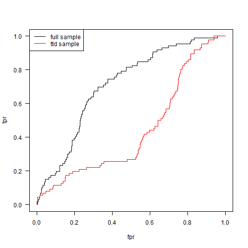
Clearly the model’s performance degrades when it’s fitted to the through-the-door sample. Note that this doesn’t always happen. Here are some ROC curves we get by running the whole process with a few different random seeds.

What to do about it?

Credit risk modellers have developed a family of techniques and rules of thumb called reject inference to deal with these issues. You still have data about rejected loan applicants, so the most basic idea is to assume that all those applicants defaulted.

In our example, we can throw in a sample of 100 rejected loan applicants, assume that they all default, and add them to the ttd data set.

u <- dat[sample(which(dat$x1 + dat$x2 >= thresh), 100),]
u$y <- 1
ttd2 <- rbind(ttd, u)

# model with reject inference
model_ttd2 <- glm(y ~. , data=ttd2, family="binomial")

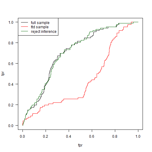
In this simple example, this fixes the problem. Real life is more complicated, of course, and there are various approaches to reject inference. The least cost-effective is just automatically approving some randomly-chosen subset of loans in order to get an unbiased data set which doesn’t suffer from rejection issues. Of course, this means that you end up approving some bad borrowers, which can be costly in the long run.

Does it arise in other fields?

There are other versions of the through-the-door problem. One amusing example is ancient credit risk data. According to The Price of Time by Edward Chancellor, Babylonian loans were recorded on clay tablets which were destroyed when the loan was fully repaid. Therefore, if you were trying to build a credit scorecard for ancient Babylon, your data set would consist entirely of defaulters!

What about applications outside credit risk? Well, surprisingly, this sort of thing comes up quite often. One recent question on Crossvalidated asks about health inspections. A health inspector wants to gather data on restaurants, but also wants to find restaurants which are likely to be violating health rules. Naturally this leads to a data set which is biased towards restaurants which are likely to be violators. This is exactly like the through-the-door problem except that the training data for your health inspection model will be biased towards “bads” rather than “goods”. You can build a machine learning model on this data but when you try to apply your model in the real world, you might get a nasty surprise!

In fact, this sort of thing happens all the time, and is a key reason why many predictive models fail. It’s always important to understand exactly how the data were collected. If the training and test data don’t come from the same population, then estimates of model performance are going to be wrong. And (unless you’re on Kaggle) the training and test data never come from the same population. That’s one reason why I prefer to evaluate models on out-of-time samples rather than relying on cross-validation!