Post-Bayesianism? Let's try it!

A recent seminar introduced me to a new kind of statistical inference called post-Bayesianism. It has its own website, seminar series, Youtube videos and, most importantly, a cool name¹. Will it catch on? I don’t know, but I think it’s interesting, and the aim of this post is to explain why I think so.

The Gibbs Posterior

One flavour of post-Bayesian inference is based on the notion of a Gibbs Posterior.

To motivate the Gibbs Posterior, first consider the usual Bayesian inference for a (possibly vector-valued) parameter $\theta$. You have a prior $\pi(\theta)$, a data set $y$, and a model which relates the two. The likelihood of your model is a function $L(y \vert \theta)$. You perform inference by getting the posterior distribution $\pi’(\theta)$, which is proportional to the prior times the likelihood

Often your model assumes that the data are obtained as an independent identically-distributed random sample of size $n$ from some probability distribution. If $p$ is the density of this distrbution, then the likelihood has the form

and the posterior distribution may be written

where

is the negative log-likelihood. Now, a Gibbs Posterior is a generalization of this. Instead of the negative log-likelihood, you can take some other loss function $\ell$ and define the Gibbs Posterior with respect to $\ell$ as

Why would you want to do this? Well, what if I tell you that you already do?

Examples

The most obvious thing you could do that’s not just the ordinary Bayesian inference is to multiply the log-likelihood by a constant $\lambda$ in Equation $\eqref{eq:1}$. This gives you a new kind of Bayesian inference in which your likelihood is raised to some power $\lambda$. This is called generalized Bayes and was the subject of the talk I attended by Yann McLachtie. Generalized Bayes is supposed to give some sort of robustness against model misspecification. The likelihood is said to be tempered or cooled, and the parameter $\lambda$ is called the temperature.

But you can think about other sorts of loss functions too. Your loss function doesn’t have to come from any sort of statistical model. It can be whatever you want. For example, there’s the whole field of Approximate Bayesian Computation, in which you consider a model whose likelihood is too complicated to write down, and you perform inference by producing simulated data sets $y’$ from your model and measuring how close they are to your data $y$, using some sort of distance function $d(y, y’)$. In this case, your loss function could just be $d$ (or something related to it) as discussed in this paper.

But there are other examples which are even closer to home!

Models and Statistics

I’ve been wanting to write down my thoughts about inference for a while. Basically I view the process as starting with something you want to know (such as the size of a whale population) and a set of vaguely-related data (such as a list of observations of whale sightings). You then build a statistical model (off-the-shelf or bespoke) to relate the two. You then use your model to calculate something about the quantity of interest.

A lot of statistics can be put into this framework, but I hit a snag when I started to think about summary statistics. For example, consider what happens when you calculate the mean of a univariate data set. You can view this as fitting a model to your data which just says that every data point has a constant value. This can certainly be useful, but it can’t be viewed as a kind of likelihood-based inference, because the likelihood of the model will be identically zero. If you think of your model as a machine which spits out a number, say $5$, and your data contains distinct values, say $(5.1, 5.2, 4.9)$, there’s no way that the model can generate your data because it can only output the sequence $(5, 5, 5)$. The probability of observing the data you observed is zero. So likelihood-based inference doesn’t work.

Everyone knows this, of course, and so we calculate the mean $\theta$ of our data set $y=(y_1, \ldots, y_n)$ by finding the minimum of a loss function, namely

(Other summary statistics like the median can be calculated in the same way using different loss functions.)

Now, one nice thing about this example is that it does fit into the Gibbs Posterior framework. Namely, if you take the prior to be $\pi(\theta) \equiv 1$ and set the temperature parameter to be $\lambda = \infty$, then the Gibbs Posterior is $100\%$ concentrated at the mean! So the notion of Gibbs Posterior somehow puts likelihood-based inference and non-likelihood-based inference on the same footing².

(That’s why I said above that you are already using Gibbs Posteriors. Maybe next time you calculate a mean, you can claim that you are “doing post-Bayesian inference in the infinite temperature realm”. Remember: it’s a question of marketing!)

Maximum Spacing Estimation and the Lone Runner

Even when the likelihood exists, it’s not always all it’s cracked up to be. My favourite example is the following: a running race is going on. The runners are numbered $1$ up to $\theta$ for some $\theta$. You happen to spot one of the runners, and it’s number $y = 37$. How many runners are there in the race?

The likelihood for this problem is the probability of observing $37$ given $\theta$, which is

This is maximized when $\theta = 37$. This is not a satisfying answer because intuitively it’s clear that something like $\theta = 2 \times 37$ would be a better guess³. Introducing a prior on $\theta$ and doing Bayesian inference doesn’t really help much, either.

In fact, the minimum variance unbiased estimator for this problem is $2y-1$ where $y$ is the runner’s number, and it can be derived using a likelihood-free method of inference called Maximum Spacing Estimation. The maximum spacing estimator doesn’t involve a statistical model, but it is calculated by minimizing a loss function, so it too fits into the Gibbs Posterior framework!

What might a post-Bayesian t-test look like?

I’m convinced that the idea of a Gibbs Posterior is mathematically elegant, but how would you actually go about using it? I really don’t know, so I decided to do some experiments using R. This is very speculative, so apologies in advance to any post-Bayesians who see this.

Let’s suppose we are given a sample dat of values from some population and we’re trying to find out about the population mean $\mu$.

dat <- c(9.5, 9.63, 9.55, 10.44, 10.55, 10.87, 10.29, 11.01, 10.18, 9.82)

Every statistican knows how to proceed. According to the seminal work of Gossett, if $s$ is the sample standard deviation, $\overline{y}$ is the sample mean, and $n=10$ then $(\overline{y} - \mu)/(s/\sqrt{n})$ follows a $t$-distribution with $n-1$ degrees of freedom. A Bayesian can view this is a likelihood for $\mu$.

But wait! That result is based on some pretty strong assumptions! Namely, that we have an IID random sample from the population and (depending on who you ask and whether $n$ is big enough) that the population is normally distributed. Maybe we’re post-Bayesians and we don’t want to make those assumptions?

What else could we do? Well, the sample mean $\overline{x}$ is the minimizer $\theta$ of the loss function

where $y_i$ are our data values. If we take a flat prior $\pi(\theta) \equiv 1$ then we can form the Gibbs Posterior

which I think will be a normal distribution with mean $\overline{y}$ and standard deviation $\sqrt{1/\lambda n}$. How do we choose $\lambda$? Well, the reason why we’re doing post-Bayesian inference is that we think our sample might not be IID. So let’s assume that we think our sample is morally equivalent to an IID sample of a much smaller size. Since $0.05$ is a popular magic number in statistics, let’s assume that our sample contains the same amount of statistical juice as an IID sample which is $0.05$ times its size. Since the $t$-distribution is close to normal, we could choose $\lambda$ so that

which means that the Gibbs Posterior is $\theta \sim N(\overline{y}, 2s^2)$.

To compare the two methods of inference, let me explain how I generated the data. I used the following sample_badly function⁴ which samples from an $AR(1)$ process. First, I drew $y_1$ from $N(10, 1)$. Then I took a sample in which each subsequent value was sampled from a neighbourhood of the previous value using an $N(0,1)$ distribution.

sample_badly <- function(n, mu, sigma, s=1){
  x <- rep(0, n)
  x[1] <- rnorm(1, mu, sigma)
  for (i in 2:n){
    x[i] <- x[i-1] + rnorm(1, 0, s)
  }
  x
}

The following code plots the posterior distributions for the two methods of inference, as well as the distribution of sample means.

set.seed(100)

# take 100 samples by sampling badly
M_bad <- matrix(0, nr=10, nc=10000)
for (i in 1:10000) M_bad[,i] <- sample_badly(10, 10, 1, 1)

xx <- seq(5, 15, len=100)
t_density <- dt((xx - mean(dat))/(sd(dat)/sqrt(10)), df=10-1)
plot(xx, t_density/(sum(t_density)*diff(xx)[1]), "l", lwd=2,
     xlab="x",
     ylab="density",
     las=1)

lines(xx, dnorm(xx, mean=mean(dat), sd=sqrt(2)*sd(dat)), "l", 
col="blue", lwd=2)

lines(density(colMeans(M_bad))$x, 
      density(colMeans(M_bad))$y, col="red", lwd=2)

\legend("topleft",
       legend=c("Naive t-test", "Gibbs Posterior", "Sample Means"),
       col=c("black", "blue", "red"), lwd=2)

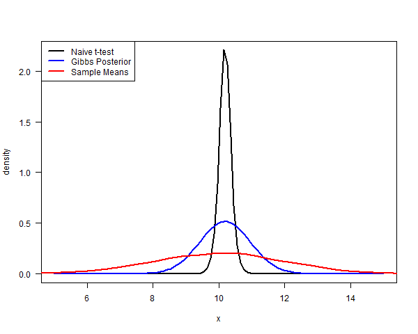
Here is what the densities look like. The plot shows the posterior distribution based on a Bayesian version of the t-statistic (with a flat prior) in black, and the post-Bayesian posterior (with a flat prior) in blue.

(Now, at this point some people might say: “But I can do better because sample_badly is just an $AR(1)$ process! I can write down the likelihood function and get the right model.” But that’s missing the point! The whole point is that you aren’t supposed to know that the data were generated by sample_badly! You were just given a suspicious-looking sample and you wanted to do inference about the population mean in a conservative way.)

The object of this exercise is to estimate the population mean $\mu$. The true value of $\mu$ happens to be $10$. For the sample dat, both the Gibbs Posterior and the Bayesian method give a reasonable-looking posterior distribution for $\mu$. What if we had taken some other sample? The red curve shows the distribution of sample means you would get if you took many different samples using sample_badly. Clearly, the Gibbs Posterior is going to do a slightly better job than the t-test, but it still isn’t conservative enough. And how could we realistically know how to choose $\lambda$ in practice? I’m not sure.

Could we get the same effect by choosing a better prior? I don’t think so. The prior expresses our uncertainty about $\mu$. But what we are really worried about in this example is our uncertainty about the sampling method itself. Bayesians have to assume that their model is $100\%$ correct, so a Bayesian who wanted to introduce model uncertainty would have to choose something like, for example, a mixture of various different models describing ways in which the sample might have been drawn. The Gibbs Posterior gives us a simpler model-free alternative.

Does it have legs?

Post-Bayesianism looks really interesting to me. Generalized Bayes can potentially give you some insurance against your model being wrong. The Gibbs Posterior can potentially cut through the whole business of building a statistical model and allow you to address the question you care about by using a loss function instead. But will this approach ever catch on?

Maybe not. The problem is that academia is mostly focussed on building models (I recall the friendly advice I got last time I tried to write a paper about prediction). If the purpose of academic papers is to impress people with your model-building skills, then is a new method of inference which assumes that your model could be wrong likely to become popular, even if gives better results? Why would someone whose job is dependent on publishing papers which show off their models want to acknowledge that their model might not be the cat’s pyjamas?⁵

Still, there can be no doubt that the post-Bayesian point of view shows that Bayesian inference, ABC, the method of moments, and other ways of fitting models to data are secretly the same thing. I think that’s really neat, and I’m looking forward to learning more about it!

Footnotes

1 Choosing the right name for things is half the battle. I spent my youth studying a subject called “quantum algebra”. I don’t deny that it’s interesting in my own right, but I also wouldn’t be completely honest if I didn’t admit that part of the draw, both for myself and for some of the other PhD students, was that it had a cool name. I’m reminded of a mathematician friend who once lamented to me: “How come when physicists generalize things they call them super and ultra but when mathematicians generalize something they call it quasi or semi?”

2 In the data profession, such as it is, a distinction is usually made between data scientists, who fit machine learning models, some of which are likelihood-based, and data analysts, who calculate statistics and build dashboards. I think this is a bit of a false dichotomy, and that the idea of a Gibbs Posterior shows that they are really the same thing. The data analysts are just using simpler algorithms to fit their models. They generally generate more marginal value and get paid less than their data scientist colleauges.

3 Don’t believe me? If you follow the maximum likelihood procedure, no matter what the runner’s number happens to be, you must conclude that it’s the maximum number in the whole field. This just doesn’t seem feasible. The problem here comes about because, although maximum likelihood has various guarantees of unbiasedness etc, those guarantees are asymptotic, so they might not work well in small samples like this one.

4 Although it looks insane, this was inspired by how the data were collected in a real-life machine learning problem which I once encountered. During model development we assumed that the data had come from a random sample. The client assumed that the method of sampling didn’t matter. We didn’t find out the truth until the project was nearly complete!

5 But maybe I’m too pessimistic? After all, Bayesianism is generally more conservative than frequentism, and it caught on eventually.