Raygun: A Bayesian Breakdown

Introduction

The Paris 2024 Olympic Games featured the debut of a new Olympic sport: break dancing. The sport made a lot of headlines after Australian competitor Raygun delivered an unusual routine which was ridiculed by many internet commentators. Is Raygun a deluded academic of the kind I have written about before? Or was she making a profoud statement about the cultural politics of break dance? I’m not qualified to say, since I know nothing about break dancing. But fortunately there are some people who are qualified to say, namely the Olympic judges. The IOC, perhaps wary of previous judging scandals, has posted all of their scores online, so I scraped them for further analysis.

Was Raygun really so much worse than the rest of the field? On a good day, could she have won a battle against any of the other competitors? Was the judging fair? Read on to find out!

Judges and Scores

Scoring System

For future reference, it’s important to understand how scoring works. The competition was decided by a series of one-on-one battles. Each battle lasted two rounds in the heats, or three rounds from the quarter-finals onwards. Each round was scored by nine judges. The judges score the competitors in five categories: Technique, Vocabulary, Originality, Execution and Musicality. Each judge produces a single number for each category. The number can range from -20 to 20. A positive number indicates that the first-listed dancer (red) was better and a negative number indicates that the second dancer (blue) was better. The scores for each judge are added up to get an overall score between -100 and 100. Each judge with a positive overall score gives one point to the red competitor. Each judge with a negative overall score gives one point to the blue competitor. The competitor with more points wins the round. The competitor who wins more rounds wins the battle.

Raygun lost all three of her heats 9-0, but we can find out more about her performance by diving into the scores in more detail.

Data

Here is an example of what the data look like:

The dancers in the pos and neg columns are red and blue respectively. So here, all of these judges preferred 671 overall, although Judge A thought Sunny was better in the categories of Vocabulary, Originality and Musicality. The NaN values in the table seem to represent zero (i.e. the judge had no preference and did not give a score in the category).

Average Score by Dancer

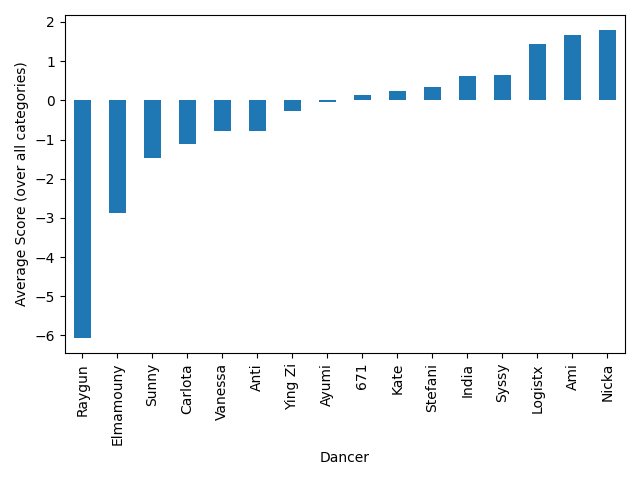
We can get a first idea of how the dancers performed by simply averaging all of their scores across all categories.

However, it’s a bit unfair to do this, since a negative score for one dancer is also a positive score for her opponent, so this gives an unfairly high score to dancers like Nicka who battled low-scoring dancers like Raygun. The overall ranking does not really reflect how the event played out. In fact, India and 671 ended up in the bronze medal match. We’ll come up with a better way of ranking the dancers below.

The Judges

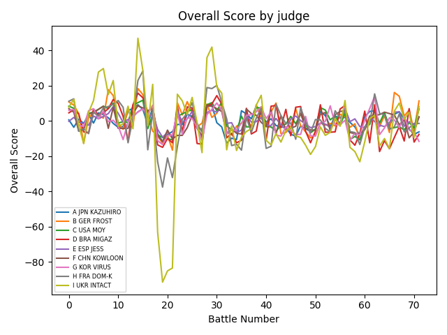
The following chart shows how each of the judges scored the dancers overall over the 72 total rounds of the competition. Remember that each score measures how much better one dancer was than the other, so the overall scores should be clustered around zero. The variance of the scores decreased as the competition went on and the weaker dancers were eliminated.

It seems that the Ukrainian judge, Intact, had strong opinions about many of the competitors, particularly Raygun, who received very low scores from him.

On the other hand, Raygun did receive positive scores from some judges in some categories (particularly the Originality category).

Assessment

I investigated the scores to see whether the categories contributed equally to the overall score. The scoring system seemed to be fair overall. The first principal component of the scores had a positive weight on each category, indicating that simply adding up the scores is likely to be a good way of ranking the dancers. The method of assigning one point per judge helps to remove the influence of very large positive or negative scores. Overall, the scoring system appeared to be fit for purpose.

However, that doesn’t tell us who the overall best dancer was. Was the gold medal awarded to the right person? How much worse was Raygun than the others?

Modelling

One question I was particularly interested in was: What if Raygun had battled one of the weakest of the other dancers, such as Elmamouny? Could she have won? If yes, with what probability? To answer this question, I turned to Bayesian statistics.

I assumed that dancer $A$ had an unknown skill level $\mu_A$ and that there was some unknown standard deviation $\sigma$ so that the scores in the battle between $A$ and $B$ were draws from a normal distribution \(s_{AB} \sim N(\mu_A - \mu_B, \sigma^2)\) Here, $s_{AB}$ is the $(9 \times \text{number of rounds}) \times 5$ matrix of scores in the battle between $A$ and $B$. This very simple model assumes that these scores (regardless of whether they represent Technique, Originality, Musicality, Vocabulary or Execution) are simply drawn from a normal distribution centred around the difference in the dancers’ skill levels.

The normality assumption isn’t really appropriate if you include Intact due to his extreme scores, so I decided just to model the other 8 judges.

The following R function simulates a battle.

simulate_battle <- function(comp1, comp2, mu, sigma, rounds=2){
  # comp1 - name of competitor who is first (+ve scores)
  # comp2 - name of competitor who is second (-ve scores)
  # mu - vector of means mu_A for each competitor
  # sigma - sd for normal distrib
  # rounds - number of rounds
  
  names(mu) <- comp
  
  # vector to store results of the rounds
  res <- rep(0, rounds*2)
  names(res) <- rep(c(comp1, comp2), rounds)
  
  for (i in 1:rounds){
    judge_scores <- rnorm(5*8, mu[comp1]-mu[comp2], sigma)
    
    comp1_score <- sum( rowSums(matrix(judge_scores, nc=5)) > 0 )
    comp2_score <- 8 - comp1_score # assume there are 8 judges
    
    res[(2*i-1):(2*i)] <- c(comp1_score, comp2_score)
  }
  res
}

The advantage of using the normal distribution is that you can write a Gibbs sampler with explicit formulas for the updates for $\mu$ and $\sigma$.

I decided to use the first competitor in alphabetical order, 671, as a reference point, so I assumed that $\mu_{671} =0$.

Inference

The following script downloads the data, temporarily removes the scores from Intact, and calculates how many scores there are for each competitor.

bgirls <- read.csv("https://raw.githubusercontent.com/rtrvale/datasets/master/olympics_bgirls.csv")

# remove scores from Intact before modelling
# (they will mess up normality assumption)
df <- bgirls[bgirls$judge != "I UKR INTACT",]

# list of competitors
comp <- union(unique(bgirls$pos), unique(bgirls$neg))

# the number of scores available for each competitor is stored in num_scores
u <- unlist(lapply(comp, function(x) length(grep(x, df$battle))))
names(u) <- comp
num_scores <- u * 5

The update for $\sigma$ uses a sample from an inverse gamma distribution

sample_sigma <- function(df, mu){
  # sample a value of sigma given mu
  # sigma ~ inv_gamma(g_alpha, g_beta)
  
  g_beta <- sum((df[,3:7] - (mu[df$pos] - mu[df$neg]))^2, na.rm=T)/2
  g_alpha <- (5 * nrow(df))/2 - 1
  sqrt( 1/rgamma(1, g_alpha, rate = g_beta) )
}

and the update for $\mu$ follows a normal distribution. If you calculate everything out on paper, some adjustments have to be made depending on whether the dancer was on the positive (red) or negative (blue) side of the battle.

sample_mu <- function(df, mu, sigma, name){
  # sample a value of mu given sigma
  
  # use first competitor ("671") as baseline
  if (name == comp[1]) return(0)
  
  # else
  pos_battles <- df[df$pos == name,]
  m_pos <- sum(mu[pos_battles$neg] + as.matrix(pos_battles[, 3:7]), na.rm=T)
  
  neg_battles <- df[df$neg == name,]
  m_neg <- sum(mu[neg_battles$pos] - as.matrix(neg_battles[, 3:7]), na.rm=T)
  
  rnorm(1, (m_pos + m_neg)/num_scores[name], sigma/sqrt(num_scores[name]))
}

Finally, these are put inside a loop in order to perform Gibbs sampling. At the same time, the results of a Raygun-Elmamouny battle are calculated at each step.

gibbs <- function(df, N, burnin=0){
  # gibbs sampler for the model
  
  mu <- rep(0, length(comp))
  names(mu) <- comp
  sigma <- 10
  
  # container for results of gibbs sampler
  res <- matrix(0, nr=N, nc=length(comp)+1)
  colnames(res) <- c(paste0("mu_", comp), "sigma")
  
  # container for results of Raygun-Elmamouny battles
  battles <- matrix(0, nr=N, nc=4)
  
  for (i in 1:N){
    for (j in 1:length(comp)){
      mu[j] <- sample_mu(df, mu, sigma, comp[j])
    }
    sigma <- sample_sigma(df, mu)
    res[i,] <- c(mu, sigma)
    
    battles[i,] <- simulate_battle("Raygun", "Elmamouny", mu, sigma)
  }
  list(res=res[burnin:nrow(res),], battles=battles)
}

Finally, here is the code to perform the inference.

set.seed(2024)
G <- gibbs(df, 10010, 10)
#samples <- G$res[10*(1:1000), ] # I decided not to thin the output
barplot(sort(colMeans(samples)[1:16]), ylim=c(-3,1), border=NA, col="skyblue", las=2, cex.names=c(0.6))

Rankings

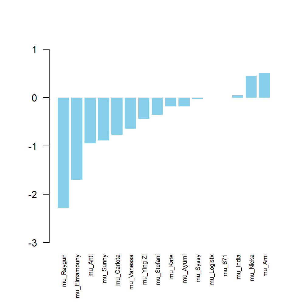
The values of $\mu_A$ for each dancer are plotted in the figure below. These values can be thought of as a skill level calculated form the ratings received rather than from the knockout system used in the actual competition.

This puts the gold medallist Ami at the top, followed by silver medallist Nicka. The next two competitiors, India and 671, battled for the bronze medal, with 671 winning. So these skill ratings do seem to give a fair reflection of the competition.

But wait! If these numbers reflect the outcome of the competition, what’s the point of calculating them at all? We have the results of the competition! Why do we need a skill level for each competitor?

Well, remember that I wanted to see how well Raygun would have performed in a theoretical battle against her closest rival Elmamouny. And we can now calculate that!

battles <- G$battles[10:nrow(G$battles),] # remove burnin
win1 <- (battles[,1] > battles[,2] + 1)
win2 <- (battles[,3] > battles[,4] + 1)
draw1 <- (battles[,1] == battles[,2] + 1)
draw2 <- (battles[,3] == battles[,4] + 1)

sum( (win1 & draw2) | (win2 & draw1) | (win1 & win2) ) # 65
sum( win1 | win2 ) # 952

(We need to remember to add in one point for Elmamouny from the Ukrainian judge.)

Raygun wins in 65 out of 1000 simulated battles. That’s a probability of 0.65%. But she does have a 9.5% chance of winning at least one round, which is significantly more than zero.

Conclusion

So, although Raygun was by far the worst competitor, perhaps she was not a total write-off. If she had battled against the second-worst, she would have had an outside chance of winning a round.

I am reminded of my own brief career as a professional dancer. This happened while I was looking for my first job after leaving academia. Despite not being very good at dancing, I was somehow selected to appear in a movie (I made the final cut, too! Tommy Lee Jones is in it!) The other dancers were wondering whether perhaps the film crew had been meaning to pick someone else with a similar name instead of me. I said to one of the film crew “You know, I’m not as good at this as the other dancers”. She replied: “Don’t worry. If everyone was really good, it wouldn’t be realistic.”

Perhaps the same could be said of the Olympic breaking final?