Double Descent Explained

This is a post about the famous double descent phenomenon in machine learning. I aim to constrct the simplest possible example of double descent and explain exactly how it arises and why it doesn’t contradict the bias-variance tradeoff.

I was inspired to write this post by an excellent video by Welch Labs entitled What the Books Get Wrong about AI. Despite the provocative title, the video explains why double descent doesn’t really mean that the books are wrong. A blog post by Alex Shtoff contains detailed Python code for an example which is similar to the one in the video.

I couldn’t find an equally good post with R code, and there seems to be a lot of misinformation about double descent online, so I thought I would write my own post. Instead of porting the Shtoff example, I also decided to create something slightly simpler. How simple can a model be but still exhibit the double descent phenomenon? To answer that, I need to explain what double descent is.

What is Double Descent?

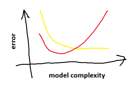
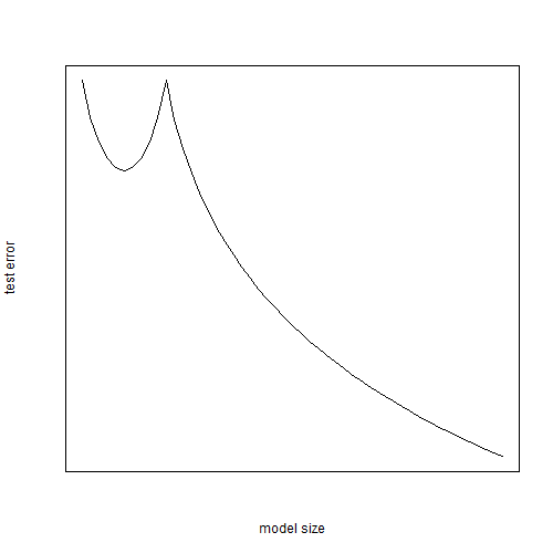
One of the key ideas in machine learning is the bias-variance tradeoff (they ask about it in every interview). This is the idea that, as a model becomes more and more complicated, it will fit the training data better and better (the yellow line in the picture below indicates the training error) but beyond some point it will become overfitted and perform worse on unseen test data (the red line in the picture indicates the test error). Since you generally want the model to perform well on unseen test data, this is a problem. It means that you need to be conservative and select a model which isn’t too overfitted.

Conceptually you should think of a U-shaped curve. You want to select the model at the bottom of the U.

As neural networks became popular, people began to notice that there’s more to it than this. As you add more and more parameters to your neural network, you see the U-shaped curve. But beyond a certain point, the test error starts going down again.

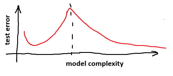
This is called double descent. As your network gets bigger and bigger, it stops overfitting. In fact, if you make the network big enough, it can even have lower test error than the model at the bottom of the U. That’s one reason why those dastardly AI companies are hoarding GPUs so that they can train models with billions of parameters. These models are just better than smaller models.

But why? What’s going on?

Data points and features

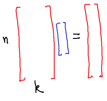
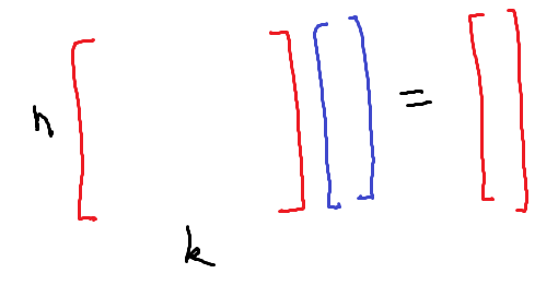
Conceptually you can think of the training data in a machine learning problem as an $n \times k$ matrix and an $n$-vector. The rows of the $n \times k$ matrix correspond to data points. The columns correspond to the values of each feature. The $n$-vector $y$ contains the desired output for each data point.

When $n > k$, you are in the traditional situation found in statistics. You have more data points than features. In this case there probably isn’t any model which fits your data exactly. You have to compromise by doing some sort of averaging process, which is roughly what linear regression does.

When $k > n$, you have too many features. In this case there will probably be many models which fit your data exactly. Most machine learning algorithms will either take some sort of average of these models, or select one of them as the best model.

When $n$ and $k$ are equal, you have exactly as many features as data points. To first order, you have $n$ equations in $n$ unknowns. There will generally be exactly one solution, so you only have one possible choice of model.

To put it another way, a machine learning problem with $n$ data points and $k$ features has roughly

degrees of freedom because this is the number of full rank submatrices in a generic $n \times k$ matrix. These degrees of freedom can be “averaged over” or exploited in some way to reduce the variance of the fitted model. Many machine learning algorithms work by adding features to an existing data set (this can also be done by hand, in which case it’s called feature engineering.) As the number of added features increases, there are more opportunities for averaging. These opportunities can sometimes be exploited to produce a better performing model.

Schematically what you expect to see is something like this:

plot.ts(-lchoose(pmax(10, 0:50), pmin(10, 0:50)), xlab="model size", ylab="test error", 
xaxt="n", yaxt="n", las=1)

This suggests that an easy way to get double descent to appear is to create an algorithm which adds randomly-generated features to a data set, which is what we will now do.

A Demo in R

We’ll generate a univariate data set with a cubic shape supported on $[-1, 1]$.

make_data <- function(n, sigma){
  x <- 2*(runif(n) - 0.5)
  y <- x * (x-0.6) * (x+0.6) + sigma * rnorm(n)
  data.frame(x=x, y=y)
}

Our model will be very simple. We’ll generate features of the form

and add them to the data. We’ll use these features to predict $y$ for new values of $x$. The following function adds the features to the data set when the values of $b$ are stored in a vector called cutoffs.

model_matrix <- function(dat, cutoffs, s_noise=0){
  n <- nrow(dat)
  N <- length(cutoffs)
  extra_features <- outer(dat$x, cutoffs, ">") + s_noise*rnorm(N*n)
  cbind(1, dat$x, extra_features)
}

In order to avoid adding two identical features, we add a small amount of noise controlled by the parameter s_noise. To include an intercept term we also add a column of ones, which is equivalent to allowing horizontally-flipped versions of the features.

To fit the model we add $K$ of these features at random. We use the Moore-Penrose pseudoinverse (the ginv function from the MASS package) of the model matrix to get a vector of regression coefficients bb. This corresponds to linear regression when $n > k$. When $n < k$ it corresponds to selecting the smallest-norm linear model which fits the data.

library(MASS)

fit_model <- function(dat, K, s_noise=0.01){
  # N is the number of random features added
  # dat is a univariate data set with columns x, y
  a <- min(dat$x)
  b <- max(dat$x)
  
  cutoffs <- runif(K)*(b-a) + a # random cutoffs

  bb <- ginv(model_matrix(dat, cutoffs, s_noise)) %*% dat$y
  list(bb=bb, cutoffs=cutoffs)
}

predict_model <- function(model, dat){
  # predict from the model from data set with column x
  model_matrix(dat, model$cutoffs, 0) %*% model$bb
}

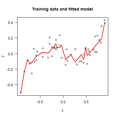
Here’s an example showing that we really can fit simulated data quite well with this model.

set.seed(2510)
dat <- make_data(50, 0.1)
model <- fit_model(dat, 20)
plot(dat, main="Training data and fitted model", las=1)
dat$pred <- predict_model(model, dat)
lines(dat$x[order(dat$x)], dat$pred[order(dat$x)], "l", col="red",
      lwd=2)

This shows the fit to the training data, but what we’re really interested in is the fit to unseen test data. We can use the following function to generate many test data sets and calculate the MSE of a pre-fitted model.

calc_test_error <- function(model, nrow_test, sigma_test, n_reps){
  
  mse <- rep(0, n_reps)
  for (i in 1:n_reps){
    dat_test <- make_data(nrow_test, sigma_test)
    pred <- predict_model(model, dat_test)
    mse[i] <- mean((pred - dat_test$y)^2)
  }
  mean(mse)
}

We also want a function to calculate the variance of each model. Here, we generate many training data sets from the same distribution and calculate the variance of the model’s predictions at each point. A higher variance means that the model is capturing more of the noise (and less of the signal) in the data.

calc_variance <- function(n_pts, n_model, sigma, n_reps){
  
  x_test <- seq(-1, 1, len=n_pts)
  fitted <- matrix(0, nr=n_reps, nc=length(x_test))
  
  for (i in 1:n_reps){
    dat <- make_data(n_pts, sigma)
    model <- fit_model(dat, n_model)
    fitted[i,] <- predict_model(model, data.frame(x=x_test)) 
  }
  mean(apply(fitted, 2, var))
}

Now everything is in place. The following code generates a data set with $10$ points and fits models with different numbers of extra features (from $0$ to $50$). Since the extra features are generated at random, each model fit is repeated several times in order to estimate the average error err on unseen test data and the average variance.

set.seed(2510)
K <- 50
model_reps <- 10
dat <- make_data(10, 0.1)
err <- vars <- matrix(0, nr=K+1, nc=model_reps)
for (i in 0:K){
  print(i)
  for (j in 1:model_reps){
    model <- fit_model(dat, i)
    err[i+1, j] <- calc_test_error(model, 100, 0.1, 1000)
    vars[i+1, j] <- calc_variance(10, i, 0.1, 1000)
  }
}

The code takes a couple of minutes to run. Here’s the final plot showing the classic double descent behaviour.

plot_col <- rep("blue", K+1)
plot_col[1:9] <- "forestgreen" # used later
df <- data.frame(vars=rowMeans(log(vars)), 
                 err=rowMeans(log(err)), 
                 plot_col=plot_col)

plot(0:K, df$err, "l", xlab="Number of added features",
     ylab="log(test error)", las=1, main="Double Descent",
     col="blue", lwd=2)
abline(v=8, lty=2, col="red")

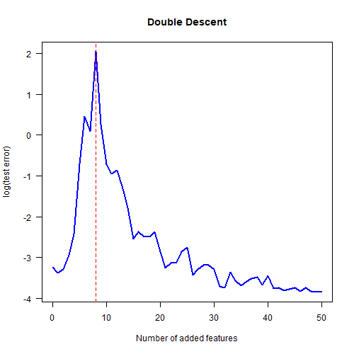
The red dotted line shows that the maximum test error occurs at $K=8$ added features. Why $8$? This is because our model matrix has $K+2$ columns and we have $10$ data points. So when $K=8$ we get a square model matrix, which means that there is exactly one possible model which can output the training $y$ values given the training $x$ values. This is the point where the maximum amount of overfitting occurs.

Note also that the models with a very large number of added features had the lowest test error; even lower than the models with just a few added features. Just like in real deep learning!

The Bias-Variance Tradeoff

The next plot shows how the variance of the model changes with the number of extra features added. Notice that this plot is the same shape as the double descent plot. As we add more features, the variance goes down.

plot(0:K, df$vars, "l", xlab="Number of added features",
     ylab="log(variance)", las=1, main="Model variance",
     lwd=2, col="darkgreen")
abline(v=8, lty=2, col="red")

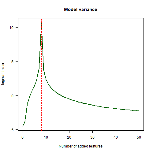
This is the key to understanding why double descent doesn’t contradict the traditional notion of the bias-variance tradeoff. When we plot the U-shaped curve in the bias-variance tradeoff, it’s the variance of the model which we should be plotting on the $x$-axis, not the “model complexity” or “model size” or some other notion of that sort.

df$K <- 0:K
df <- df[order(df$vars), ]
plot(df$vars, df$err, col=df$plot_col,
     pch=19, xlab="log(variance)", ylab="log(test error)",
     las=1, cex=1.3)

loess_fit <- loess(df$err ~ df$vars, span = 0.6)
lines(df$vars, predict(loess_fit), col=rgb(0, 0, 0, 0.1), lwd=10)

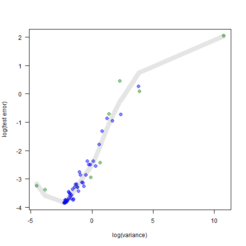
When we plot the test error against the variance, we do get the familiar U-shaped curve after all. The green points are the models which are below the $K=8$ threshold. The blue points are the models which are above the threshold. Together they form a nice familiar pattern.

The Lottery Ticket Hypothesis

This simple example illustrates some ideas about deep learning. A lot of research is currently devoted to the question of why deep neural networks are so effective in practice. One idea which has been suggested is the so-called lottery ticket hypothesis. This postulates that a deep neural network initialised with random weights is essentially calculating a large number of random features, just like the model above. Just by chance, some of these features are likely to be useful for prediction. The process of training the network tends to promote these useful features, leading to an effective model. The larger the network, the more random features are created, and the higher the chance that some of them will end up being useful.

(As usual, though, the devil is in the details. If we increased the dimension of our data set in the example above, we’d quickly discover that our random features will be zero almost everywhere. The very clever way deep neural networks are set up makes this unlikely to happen in the neural network case, but that’s a topic for another day.)

Anyway, I hope this post has convinced you that double descent is not so mysterious (it emerges from just a few lines of R code) and that the bias-variance tradeoff is very much alive!