Gladiator Simulator, Part II
by Richard in30 Apr 2020
This is a follow-up to the previous post, in which I was interested in simulating a fight between two groups of gladiators, each of whom does a random amount of damage to the other group at each time step.
This resulted in the following model with $a_0, b_0, p, q > 0$ and $\mathrm{Bin}(N, \pi)$ being notation for a binomial random variable.
\[\begin{align*} a_{n+1} &= \mathrm{max}(0, a_n - \mathrm{Bin}(b_n, q))\\ b_{n+1} &= \mathrm{max}(0, b_n - \mathrm{Bin}(a_n, p)) \end{align*}\]I am interested in which side is more likely to win, what the winning probability is, and how many survivors there will be on the winning side.
It is easy enough to simulate, but I am particularly looking for an analytic solution.
Lanchester’s Law
I mentioned previously that the model may be connected to Lanchester’s Law, a law about fighting which states that the quantity
\[pa_n^2 - qb_n^2\]should be a constant. It is possible to get a partial solution to the gladiator model by using this idea.
The starting point is to consider
\[p a_{n+1}^2 - q b_{n+1}^2 = p(a_n - \mathrm{Bin}(b_n, q))^2 - q(b_n - \mathrm{Bin}(a_n, p))^2\]and expand the right hand side, to get
\[pa_n^2 - 2pa_nY_n + pY_n^2 - qb_n^2 + 2qb_nX_n - qX_n^2\]where $X_n \sim \mathrm{Bin}(a_n, p)$ and $Y_n \sim \mathrm{Bin}(b_n, q)$ are independent. The expected value of $pY_n^2 - qX_n^2$ is
\[E[pY_n^2 - qX_n^2] = pE[Y_n^2] - qE[X_n^2] \approx pq^2b_n^2 - qp^2a_n^2 = -pq(pa_n^2 - qb_n^2)\]using that $a_n^2$ and $b_n^2$ are much bigger than $a_n$ and $b_n$ respectively. Therefore,
\[p a_{n+1}^2 - q b_{n+1}^2 \approx (1-pq)(pa_n^2 - qb_n^2) - 2pa_nY_n + 2qb_nX_n\]plus another term with zero expected value (but positive variance). Neglecting this term and using the normal approximation to the binomial yields the approximation
\[p a_{n+1}^2 - q b_{n+1}^2 \approx (1-pq)(pa_n^2 - qb_n^2) + N(\mu_n, \sigma_n^2)\]where $\mu_n = 2qb_nE[X_n] - 2pa_nE[Y_n] = 0$ and $\sigma_n^2 = 4q^2b_n^2\mathrm{Var}(X_n) + 4p_n^2\mathrm{Var}(Y_n)$.
Writing $a=a_0$, $b=b_0$ and assuming that $pq$ is small enough that $(pq)^2 \approx pq$ and that $a_n$ is much less than $a_0$ and $b_n$ is much less than $b_0$, we get that at time $t$, when the battle ends,
and note that at time $t$, by definition, we must have one of $a_t$, $b_t$ equal to zero. The probability of side $A$ winning is the probability that $X:= N((1-pq)(pa^2 - qb^2), \sigma^2)$ is positive, and the number of survivors $a_t$ satisfies $pa_t^2 \sim X$, given that $X > 0$.
Performance
Now I want to do some simulations to test the accuracy of $\eqref{eq:1}$, given that we have made some dodgy approximations in order to get it. The graph shows the results of pitting $b$ gladiators with kill probability $q$ against $a=100$ gladiators with probability $p=0.5$. The red curves are the simulation results and the blue curves are calculated from $\eqref{eq:1}$. The value of $q$ ranges from $1$ for the leftmost curve to $0.1$ for the rightmost curve. Loss probability for side $B$ (with the variable number of gladiators) is plotted on the $y$-axis.
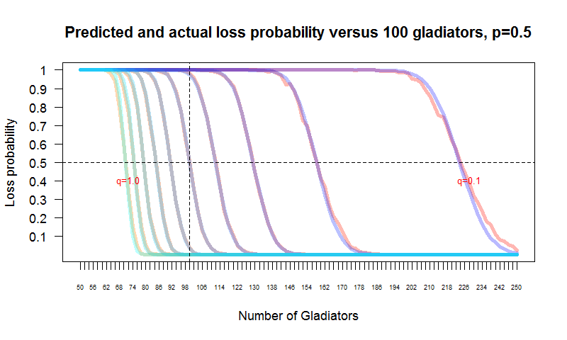
From the graph, it looks like $\eqref{eq:1}$ gives a very good estimate of probability of a win or loss for a particular side.
Survivors
Looking at the survivors in the case $a=20, b=10, p=q=0.5$ (discussed in the previous post) the fitted distribution looks pretty good. The graph shows the result of 10000 simulations.
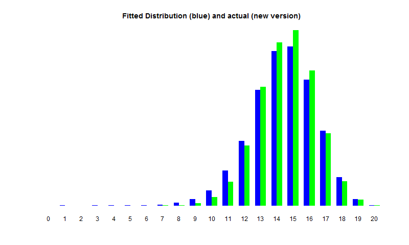
However, the story is rather different when we look at a range of different values of the paramaters. The predicted distribution of survivors can end up being in completely the wrong place.
The next two graphs show the result of simulations, colour coded by the value of the probability $q$. For each value of $q$, the difference between the predicted mean number of survivors on the winning side given by $\eqref{eq:1}$ and in average survivors from 1000 simulations is plotted, first versus the value of $b$ and then versus the value of $q$.
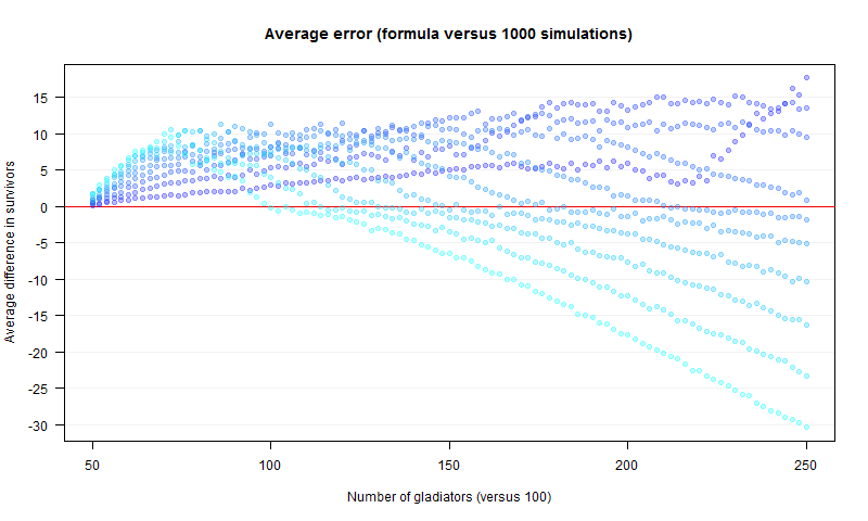
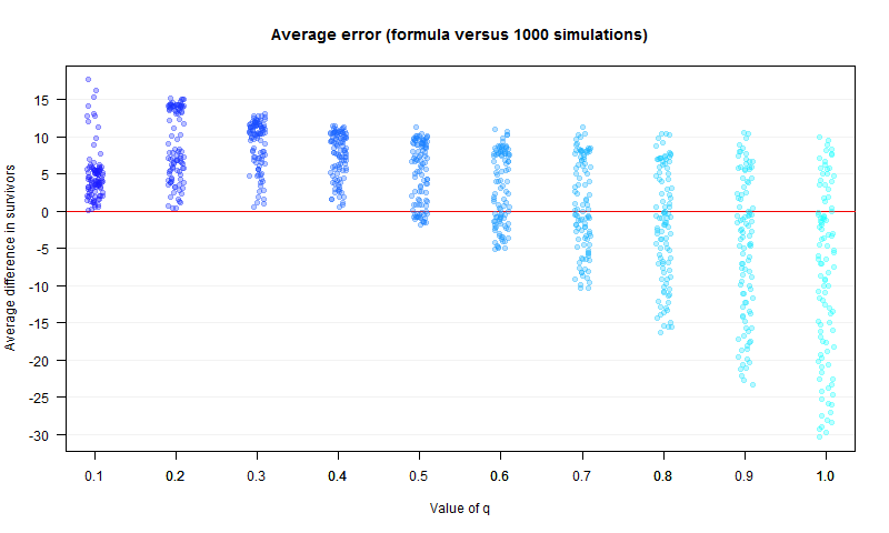
It is clear that some of the approximations used to get $\eqref{eq:1}$ were a bit too cavalier, and $\eqref{eq:1}$ does not tell the whole story.
Related Work
While searching for references about this model, I came across a surprisingly recent paper by Kearney and Martin on the arXiv, which discusses stochastic Lanchester models. Kearney and Martin present formulas for the probability of one side winning and the number of survivors which are similar to $\eqref{eq:1}$. However, their model is different.
In the stochastic Lanchester model considered by Kearney and Martin, only one gladiator dies at each time step, with the side of the unlucky gladiator being chosen with probability $qa/(pb+qa)$. (They also work out what happens with more general functions in place of this one). This means that once one side has shrunk, it has a much lower chance of getting any future hits on the other side, whereas in the model considered in this post, even the smallest force can still do some damage.
Taking things one gladiator at a time means that the model can be viewed as movement along a lattice and there is a huge amount of mathematical theory which can be applied to it.
I am not sure which model I think is more realistic; they both have their points and result in very similarly-shaped distributions of survivors and survivor probability curves.