Jigsaw Equation

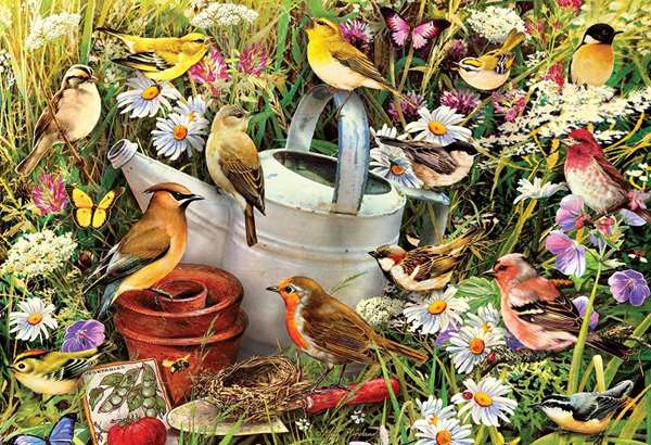
The picture below shows Hidden Hideaway, a 500-piece jigsaw puzzle published by Gibson’s Games. In this post I propose to show, using nothing but some questionable mathematics and some even more questionable image processing, that Hidden Hideaway is, in some sense, the ultimate jigsaw puzzle. How? Read on!

While completing a jigsaw puzzle recently, it occurred to me that much of it ultimately comes down to trial and error. It is possible to sort pieces into different types such as edge pieces, pieces of a similar colour, etc, but at some point you are left with a pile of pieces which all show sky, for example, and the only way to complete that part of the puzzle is to try them in every possible configuration until you find one that fits.

In the extreme, a plain jigsaw with no picture at all would be very boring. But a jigsaw with a picture that is too busy would also suffer from the same problem. For example, if all the pieces were a different colour then it would require just as much trial and error as a blank puzzle, and if the puzzle showed a completely random picture, it would probably be almost (but perhaps not quite) as bad. For example, this jigsaw does not appeal to me very much.

I wondered if somewhere in between these two extremes, there was an optimum, at which the amount of trial and error required to solve the puzzle is minimized.

Model

Let us assume we have a jigsaw puzzle with $N$ pieces, which is divided into $b$ sections or blocks, where the $i^{th}$ block consists of $n_i$ pieces. The pieces within each block are assumed to have the same colour or pattern, and the different blocks are assumed to be distinguishable from each other.

Ignoring the geometry of the situation, let us treat the task of reconstructing the puzzle as arranging the pieces in a row. Assume we can quickly sort the pieces by colour, but we have to use trial and error to decide how to arrange pieces of the same colour, and also to decide how to arrange the blocks relative to each other

The blocks can be permuted among themselves in $b!$ ways, and (ignoring orientations) there are $n_i!$ ways of permuting the pieces in the $i^{th}$ block. So, altogether, the number of possible configurations (or roughly, the amount of trial and error required (or thermodynamic probability, as I believe it is called in statistical mechanics)) is

and we would like to minimize this, subject to the condition $\sum_{i=1}^b n_i = N$.

For example, in the diagram below, there are 3 blocks which can be arranged in $b!=6$ possible ways, and within each block, there are $5!=120$ ways of arranging the green pieces, $3!=6$ ways of arranging the blue pieces, and $4!=24$ ways of arranging the red pieces, giving a total of $6 \times 24 \times 120 \times 6$ possible arrangements.

 

The two extreme cases are $b=1, n_1=N$, which corresponds to a blank picture, and $b=N, n_i=1$ for all $i$, which corresponds to randomly-coloured pieces. Both of these cases give a score of $N!$.

To find a minimum in between, it is better to allow everything to be continuous and take the logarithm, so that we can define

which we would like to minimize subject to $\sum_{i=1}^b n_i =N$.

Notice that this is not a conventional calculus problem because $b$ is allowed to vary as well as the $n_i$. However, at a global minimum, regardless of the value of $b$, all the $n_i$ have to be equal. This is because if $n_i < n_j$ for some $j$, then there is some $\varepsilon$ with $n_i + \varepsilon < n_j - \varepsilon$ and then

where $\psi$ is the digamma function. Because $\psi(n_i) < \psi(n_j)$ ($\psi$ is an increasing function; in fact $\psi(x)$ resembles $\log(x)$) we would not have a global minimum.

Therefore, we can assume all the $n_i$ are equal, and since they add up to $N$, we can put $n_i = N/b$ for all $i$. Then

and now we can let $b$ vary and minimize this using calculus, which gives the equation

Recap: the claim is that the amount of trial and error in assembling an $N$-piece jigsaw will be minimized if it is divided into $b$ sections of equal size, where $b$ is related to $N$ by $\eqref{eq:1}$.

Approximate solution

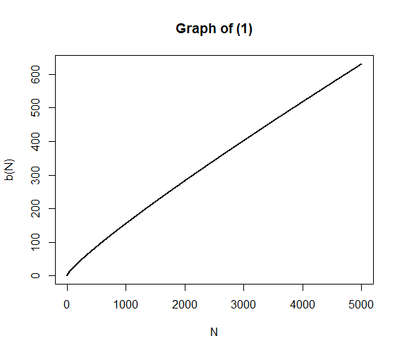
A few lines of R can be used to make a graph of $\eqref{eq:1}$, from which it appears that $b$ doesn’t vary very spectacularly with $N$.

j <- function(b, N) lgamma(N/b+1) - (N/b)*digamma(N/b+1) + digamma(b+1)
y <- N <- 1:5000
for (i in 1:5000) y[i] <- uniroot(function(b) j(b, N[i]), c(0.1, N[i]))$root
plot(N, y, "l", ylab="b(N)", main="Graph of (1)", lwd=2)

I am particularly interested in the cases of a 1000-piece puzzle, for which $b=155.6$ and a 500-piece puzzle, for which $b=86.36$. This corresponds to sections of size 6.4 and 5.8 respectively, so our jigsaw puzzle should be divisible into blocks of about 6 pieces each. In terms of the picture, this would correspond to a picture which contains a large number of small and easily-distinguishable items or regions, in other words, something graphically “busy”.

I have not been able to find a way to simplify $\eqref{eq:1}$, but at least it is possible to find an approximate solution, depending on what counts as a solution.

From Stirling’s Formula, we have $\log\Gamma(x+1) \approx x\log(x) - x + \frac{1}{2}\log(2\pi x)$. Furthermore, $\psi(x+1) = \psi(x) + 1/x$ for all $x$, and also $\psi(x) \approx \log(x) - \frac{1}{2x}$ is a very good approximation for $x > 1$. If we put $x=N/b$ in $\eqref{eq:1}$, it simplifies down to

which after rearrangement gives

Now, it so happens that $f(t) = te^t$ has an inverse called $W$, and so using this so-called Lambert W-function, we can get

which, recalling that $x=N/b$, gives our approximate solution to $\eqref{eq:1}$ as

How good is the approximation? Well, it looks pretty good graphically, in the sense that adding it in to the previous graph, in blue, it matches up quite well with the graph of $\eqref{eq:1}$.

y2 <- y
for (i in 1:5000) y2[i] <- (2*N[i]-1)/uniroot(function(b)b*exp(b) - 
2*pi*exp(-1)*N[i]*(2*N[i]-1), c(0.1, N[i]))$root
lines(N, y2, col="blue")

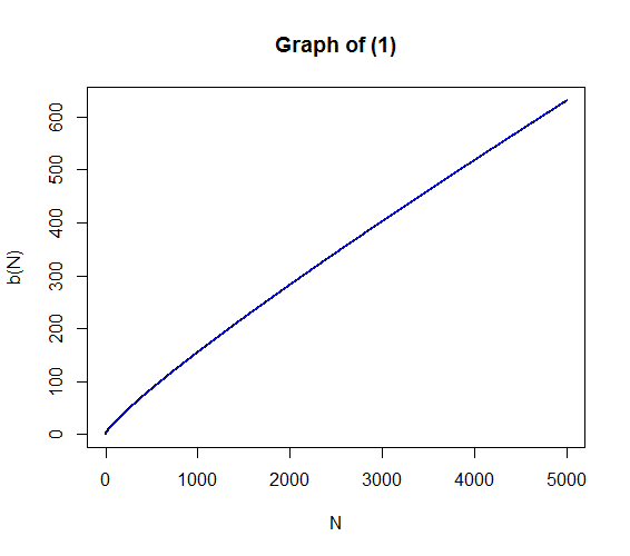
but it is a little off and, of course, we don’t really need it, since we can solve $\eqref{eq:1}$ easily enough using the bisection method. (Still, I think it’s nice to have a formula).

Application to real puzzles

Having determined what a good jigsaw puzzle ought to look like, I wanted to search for real puzzles which are as close as possible to satisfying $\eqref{eq:1}$. Of course, it’s not obvious how to do this, which is where the questionable image processing comes in.

Step 1: Find some puzzles

After some searching, I found a mail order site, Jigsaw Puzzles Direct, with a convenient page listing all of their jigsaw puzzles, with links to images. I am new to web scraping, but this seemed like a good place to start. I used the following code to make a list of links to all of the images.

import re
import BeautifulSoup
# get the urls of the images to be evaluated
url = '''https://www.jigsawpuzzlesdirect.co.uk/jigsawchoice.asp?sort=&subpieces
      =&subpicture=&subcharacter=&subage=&subartist=&submanufacturer=&assistantsubmit
      =Find+your+perfect+puzzle%21'''
response = requests.get(url)
soup = BeautifulSoup.BeautifulSoup(response.content)
images = soup.findAll('img')
sources = [x['src'] for x in images]

# use a regex to get the jpg files only (for the products)
regex = re.compile(r'.*productssmall.*\.jpg')
selected_files = filter(regex.search, sources)

# convert everything to the large size image file format
jpgs = []
for i in range(len(selected_files)):
    x = selected_files[i].encode('ascii', 'ignore')
    #print(x)
    x = str.replace(x, '/productssmall', 'https://www.jigsawpuzzlesdirect.co.uk/prodhuge')
    x = str.replace(x, ' ', '')
    jpgs +=[x]
    
# jpgs contains the urls for all the images whose complexity is to be evaluated

Step 2: Process the images

Having got these image files, I processed each of the images as follows. First, I divided each image into rectangles, keeping the ratio of height and width. (This is how it is done for real jigsaw puzzles; it is common for puzzles not to have the exact number of pieces which it says on the box). The following code fragments use various libraries, including PIL.

im = Image.open(image_file)
        
# get width and height of image for re-scaling
width, height = im.size
puzzle_width = int(round(sqrt(n_pieces * width / height)))
puzzle_height = int(round(sqrt(n_pieces * height / width)))

Next, the image is rescaled, so that there is one RGB pixel per puzzle piece. The colours of these pixels are stored in a numpy array.

# resize to desired jigsaw size
puzz = im.resize((puzzle_width, puzzle_height))
        
# pixel colours
pixel_values = numpy.array(list(puzz.getdata())).reshape(n_pieces, 3)  

I then took the first principal component of the RGB colours. This process projects each RGB pixel colour to a one-dimensional line, chosen in such a way that the variance of the projections is maximized.

# get the first principal component of the RGB colours in the image
from sklearn.decomposition import PCA
pca = PCA(n_components=1, svd_solver='full')
pca.fit(pixel_values)
fpc = pca.transform(pixel_values) # first principal component
out = []
for i in range(n_pieces):
    out += fpc.tolist()[i]

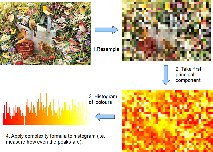
I then made a histogram of these values with the number of equally-spaced bins given by $\eqref{eq:1}$ (155 for a 1000-piece puzzle and 86 for a 500-piece puzzle). From this histogram, we get the count for each bin, and the complexity of the puzzle was taken to be the complexity of this vector of counts.

def complexity(x):
    """calculate the complexity of a vector x, using the formula
    sum_i log (gamma(x[i] + 1)) + log(gamma(length(x)+1))"""
    total = 0
    for i in range(len(x)):
        total += scipy.special.gammaln(x[i]+1)
    total += scipy.special.gammaln(len(x)+1)
    return total  

# split into equal parts
x = numpy.histogram(out, puzzle_sections)[0].tolist()
complexity(x)

This diagram summarizes the process. Computing the complexity is really just measuring how close the peaks in the histogram are to being all the same height.

For the 1000-piece puzzle, here are the top ten images (meaning, the ten images with the lowest complexity values when $N=1000$ and $b=155$). Note: I am linking to the images, so they are likely to change or disappear over time. Notice that one of the images is actually a picture of a box rather than of the puzzle itself. This is a problem of course, but it did not seem worth doing extensive cleaning of the images, given the crudeness of the image analysis.

Here are the top ten images for a 500-piece puzzle ($b=86$).

The same images kept cropping up, even when I ran the algorithm with the wrong parameters. Probably, these are the images which have the most even spread of colours among all images considered, so perhaps there is not too much to be read into this. But, for what it’s worth, Hidden Hideaway tends to come out at the top. As promised!

(Recall once more what this means. The claim is that, out of all the pictures considered, the picture on Hidden Hideaway requires the least amount of trial and error to reconstruct when it is divided into a 1000 or 500-piece jigsaw. If trial and error is the least interesting aspect of assembling a jigsaw, then Hidden Hideaway is the most interesting puzzle).

Comments

It occurred to me that what I called complexity should probably be called entropy, because it is the logarithm of the number of possible configurations. This leads me to think that equations $\eqref{eq:1}$ and $\eqref{eq:2}$ could well have cropped up somewhere in statistical mechanics, but unfortunately I am not familiar enough with the subject to know where to look. Also, I understand that physicists usually want to maximize entropy, whereas I was trying to minimize it.