Board Game Group EDA
by Richard in30 May 2019
Until moving country recently, I was regularly attending a very well-organized local boardgame meetup. The people who run the group make a weekly list of the attendees and the games they played, all of which is stored in a publicly-accessible Google spreadsheet. They have been doing this for long enough that a reasonable amount of data has built up, of which there is slightly too much for comfortable hand-prcoessing.
The spreadsheet has one sheet for each week of data. The individual sheets look like this (I have edited the names):
Below the name of each game is a list of the players. The format is fairly consistent from week to week.
There are many possible approaches for ingesting these data. In retrospect, a good approach might have been to get a list of all the possible board games from a database such as Boardgamegeek, and then add the player names by finding the games in the sheets. The problem with this method is that some game names vary, for example because of multiple games being played at once, or games being played with expansions.
My approach was to look for the cells containing an F_ or O_ (indicators which are used to show whether a game is full (has its full complement of players) or open (more players can join)). Above each F_ or O_ is the game name, and below is the list of players. This method will omit some games, such as Spirit Island in the above example, but generally works quite well.
The sheets are read into R using the very nice readxl package and processed using the following code. The output of the function is a list indexed by the games played on each date, with the number of players (if it was given as a single number) and the player names (if a valid number of players was found). For some games, such as Puerto Rico in the above example, this method will not record the players who played the game, but this does not matter, since my main interest was in which games were played.
# function for getting the info from a single sheet
process_sheet <- function(sheet){
  # sheet should be a data frame

  # find the cells which contain F_ or O_
  full_open <- which(sheet=="F_" | sheet=="O_", arr.ind=T)
  game_list <- list()
  for (i in 1:nrow(full_open)){
    #print(i)
    idx <- full_open[i, ]
    name_idx <- idx + c(-1, -1)
    game_name <- sheet[name_idx[1], name_idx[2]]
    z <- idx + c(0, -1)

    # number of players, if given
    n_players <- as.numeric(gsub("Players", "", sheet[z[1], z[2]]))

    # if number of players was given, create a list of player names
    if (!is.na(n_players)){
      player_names_idx <- matrix(rep(idx, n_players), nc=2, byrow=T) + cbind(1:n_players, -1)
       player_names <- sheet[player_names_idx[1, 1], player_names_idx[1,2]]
      for (i in 2:n_players){
        player_names <- c(player_names, sheet[player_names_idx[i,1],
                                            player_names_idx[i,2]])
      }
      player_names <- player_names[!is.na(player_names)]

      # if any player names were found, add them to this
      # recorded play
      if (length(player_names) > 1){
        game_list[[game_name]] <- list(n=n_players, player_names=player_names)
      }
    }
  }
  game_list
}
After some further processing, the output was turned into a list of games played in each week, from which I obtained a matrix whose rows were the 66 weeks and whose columns were the games played. Even after some cleaning of the game names, there were still 289 recorded games.
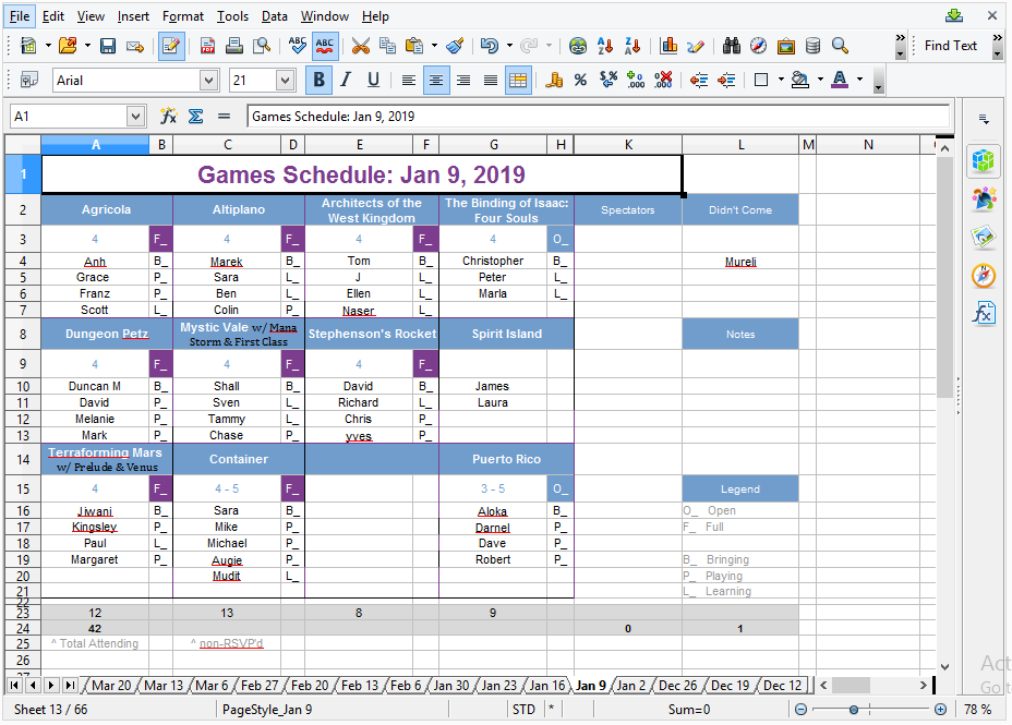
The image below shows the matrix of games played by week, with games along the horizontal axis and time on the vertical axis (going downwards from week 1 to week 66). The games are ordered by decreasing number of plays. Most games are played once and then never seen again. This fate befell 201 of the 289 games, almost 70% of the total.
I was interested in ranking the remaining games by popularity. Simply counting the number of plays is not sufficient because we should also consider the amount of time which has elapsed since a game was last played. The plays of each game can be considered as a binary time series, and the simplest model for such a series is a logistic regression with time as the dependent variable. My idea was that the overall trend in the popularity of a game could be measured by the coefficient of time in the logistic regression, and the current popularity could be measured by the probability that it will be played next week.
Each logistic regression starts from the first time a game was played, in order to make a fair comparison between games.
n_weeks <- 66
container <- rep(NA, ncol(game_matrix))
names(container) <- colnames(game_matrix)
pred_prob <- lr_slopes <- se_slopes <- se_pred <- container

for (i in 1:ncol(game_matrix)){
  x <- game_matrix[,i]

  # start at the first time the game was played
  first <- which(x==1)[1]
  x <- x[first:length(x)]
  t <- first:n_weeks
  model <- glm(x ~ t, family="binomial")
  pred <- predict(model, data.frame(t=n_weeks+1), se.fit=T,
                  type="response")

  # beta (coefficient of t) in logistic regression model
  lr_slopes[i] <- coef(model)[2]

  # standard error of beta
  se_slopes[i] <- sqrt(diag(vcov(model)))[2]

  # predicted probability of being played next time
  pred_prob[i] <- pred$fit

  # standard error of the prediction
  se_pred[i] <- pred$se.fit
}
Note that many of the logistic regressions do not converge. These are precisely the ones for which a game was played in some consecutive number of weeks and at no other time, so that its time series of plays looks like 1 1 1 0 0 ... 0. These give perfectly separable logistic regression data. As a special case, this includes all games which were only played once.
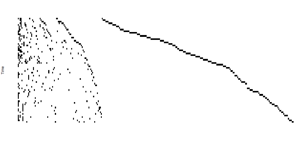
We can visualize the popularity of the top six most played games over time.
par(mfrow=c(2,3))
for (i in 1:6){
  plot.ts(game_matrix[,i], axes=F, ylab="", main=colnames(game_matrix)[i])
  x <- game_matrix[,i]

  # start at the first time the game was played
  first <- which(x==1)[1]
  x <- x[first:length(x)]
  t <- first:n_weeks
  model <- glm(x ~ t, family="binomial")

  pred <- predict(model, data.frame(t=t), type="response")
  lines(t, pred, col="blue", lwd=3)
}
par(mfrow=c(1,1))
Terraforming Mars (a game which I have never actually played) is the only game which has remained perennially popular. However, it is not the only game with a positive coefficient of t in logistic regression. Any game played in the most recent week (week 66) is also very likely to have a positive coefficient, because the logistic model will be swayed by the most recent result when there is not much data.
We can partially avoid this problem by only looking at games which have been played 3 or more times, of which there are 40. Looking at the probability of these games being played in the next week, the top 10 are as follows.
| Game | Pr(played in week 67) |
|---|---|
| Terraforming Mars | 0.67 |
| Pandemic Legacy Season 2 | 0.38 |
| Coimbra | 0.27 |
| Castles of Mad King Ludwig | 0.11 |
| Great Western Trail | 0.07 |
| Scythe | 0.07 |
| Tramways | 0.05 |
| Transatlantic | 0.05 |
| Mystic Vale | 0.05 |
| Orleans | 0.04 |
The only ones of these which were actually played in week 67 were Terraforming Mars (twice!) and Coimbra, along with a different version of Pandemic, which doesn’t count.
Clearly, it doesn’t make sense to build a separate model for each game, since there is a limit to the number of games which can be played in any given week, and therefore, if one game is played, it influences the probability that others are played. Thus, it would be more correct to model the joint distribution of the games that are played, as I did in my Game of Thrones model.
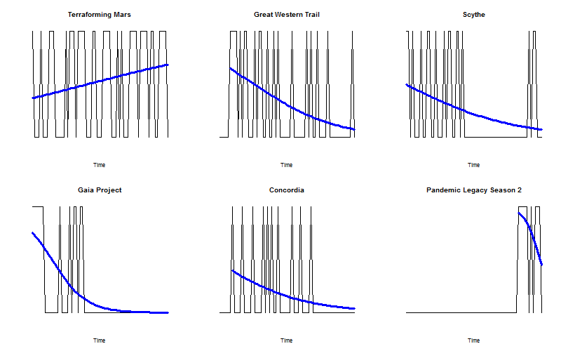
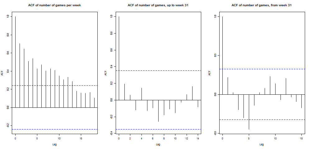
This can get very complicated, and does not seem appropriate for an exploratory analysis. However, it does suggest that it might be interesting to look at the number of games played per week. The number of games played per week has a surprisingly glaring breakpoint at week 31, with a mean of 10.6 games beforehand and a mean of 6 games afterwards.
Before and after week 31, the number of games behaved like white noise, as is suggested by the following autocorrelation plots.
The number of new games per week follows a similar pattern, with an average of 2.5 new games per week from week 31 onwards. As it happens, in week 67 two new games were played (Pandemic: Fall of Rome, and Musuem) along with two previously-played ones (Age of Steam and Egizia) and Terraforming Mars and Coimbra, as mentioned above.