Solving a regression puzzle with a custom perceptron
by Richard in10 Aug 2021
I was recently asked to solve a linear regression problem for a friend of the wife of a colleague. The problem statement, shared via Whatsapp, was as follows.
想問下如果數據x, y_lo, y_hi, error function: if y_lo <= estimate_y <= y_lo, error=0 if estimate_y < y_lo, error=y_lo-estimate_y if y_hi < estimate_y, error = estimate-y_hi
點樣穩返條直線出來?
應該係甘講, 每個x會有兩個y, y_lo同y_hi. 是終出來果條線要盡量多係y_lo同y_hi之間穿過
The process has several steps.
-
Rewrite the question to get a precise problem statement
-
Experiment with some examples
-
Find the right technique for solving the problem
-
Produce a solution
-
See if there is a simpler solution after all
Step 1
The first step is to write a precise problem statement.
The question asks for a straight line $\hat{y}=mx+c$, and it’s clear that it is a kind of linear regression. The difference is that, instead of a single $y$ value for each $x$, there are two $y$-values, $y_{lo}$ and $y_{hi}$.
Here is an example of the set-up.
The question asks for a linear error, but I expected that, if this was meant to be a generalization of linear regression, squared error was actually required. So I decided to answer the following question.
Given $x_i, y_{i, lo}, y_{i, hi}$, $1 \le i \le n$, $y_{i, lo} < y_{i, hi}$, find $m$ and $c$ which minimize
\[\sum_{i=1}^n \left((y_{i, lo} - mx_i - c)^2 \delta_{mx_i + c < y_{i, lo}} + (y_{i, hi} - mx_i - c)^2 \delta_{mx_i + c > y_{i, hi}}\right)\]Because the unknowns appear in the Kronecker delta, I can’t see a way to solve this directly using calculus. Therefore, it seems that some sort of algorithm will be required (although see Step 5 below).
Step 2
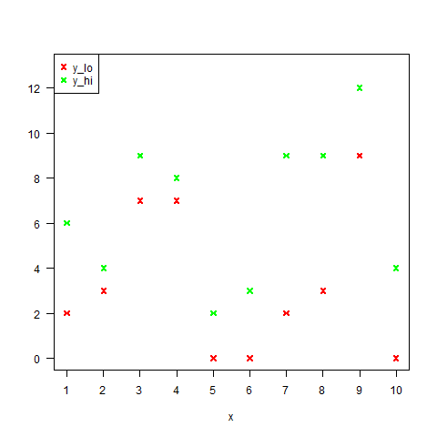
It is desired to find a line which minimizes the sum of the squares of the blue distances in the following figure.
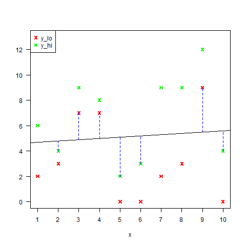
After plotting some examples with $y_{i, lo}$ and $y_{i, hi}$ in different colours, I realized that this can be interpreted as finding a decision boundary between two data sets.
Namely, one data set is ${ (x_i, y_{i, lo}) }$ (the red points) and the other is ${ (x_i, y_{i, hi}) }$ (the green points). We need to find a straight line which separates these if possible. If not, then we need to find a straight line which minimizes the error.
As an explicit example, suppose we have the following table of values of $x$, $y_{lo}$ and $y_{hi}$.
| x | y_lo | y_hi |
|---|---|---|
| 1 | 0 | 4 |
| 2 | -1 | 1 |
| 3 | 3 | 4 |
Define a new data set by
| a | b | z |
|---|---|---|
| 1 | 0 | -1 |
| 2 | -1 | -1 |
| 3 | 3 | -1 |
| 1 | 4 | 1 |
| 2 | 1 | 1 |
| 3 | 4 | 1 |
Then we want to find a way to separate the points ${(a_i,b_i)}$ in the two classes defined by $z$, which can be done, for example by using logistic regression. In our case, we want to find a particular separating line which minimizes our error function.
Step 3
The problem of finding a separating line between two classes reminded me very strongly of the Support Vector Machine. But it doesn’t seem that this problem is quite the same as the SVM optimization problem.
After some searching, I remembered that the perceptron is an algorithm which finds the separating hyperplane which minimizes the sum of squared distances from the misclassified points to the separting hyperplane.
This is almost what we want, because a misclassified point is precisely a point which is on the wrong side of the line, and these are the points which appear in the loss function from Step 1. The only difference is that we only want to minimize the vertical distance, rather than the square of Euclidean distance.
The error function to be minimized becomes
\[f(m, c) = \sum_{i \textrm{ misclassified}} (mx_i + c - y_i)^2\]where the sum is over the misclassified points. The gradient is
\[\nabla f = 2\sum_i (mx_i + c - y_i) (x_i, 1)\]and the update is $(m, c) \mapsto (m, c) - \lambda \nabla f$ where $\lambda$ is a small number. By iterating these updates, we will eventually reach a local minimum in the same way as for the perceptron.
Step 4
The perceptron can be implemented in the following way. It is written in terms of points ${ (a_i, b_i) }$ and targets ${ y_i }$ with $y_i \in { -1, 1 }$. This implementation checks whether each of the cardinal directions produces an increase in the error to decide whether a local minimum has been reached.
vertical_perceptron <- function(a, b, y,
                                learning_rate=1,
                                discount_factor = 0.9,
                                n_its=1000,
                                start=c(1,1),
                                tol=0.001){

  # version of the perceptron which minimises vertical distances between
  # boundary line and points
  # a : a vector of length m (x-values)
  # b : a vector of length m (y-values)
  # y : a vector of length m, entries are -1 or 1 (classes)
  # n_its : number of times to iterate through all m points
  # start : start value for betas

  error <- function(a, b, y, betas){
    # prediction
    bhat <- betas[1] + betas[2]*a

    # b is above the boundary but prediction is negative class
    err1 <- (bhat < b) & (y < 0)

    # b is below the boundary but prediction is positive class
    err2 <- (bhat > b) & (y > 0)

    # sum of squared prediction errors
    sum((bhat - b)^2 * (err1 + err2))
  }

  betas <- start

  for (it in 1:n_its){
    # get current error
    err_current <- error(a, b, y, betas)
    #print(err_current)

    # prediction
    bhat <- betas[1] + betas[2]*a

    # b is above the boundary but prediction is negative class
    err1 <- (bhat < b) & (y < 0)

    # b is below the boundary but prediction is positive class
    err2 <- (bhat > b) & (y > 0)

    grad1 <- sum( (bhat - b) * (err1 + err2) * 2 )
    grad2 <- sum( (bhat - b) * a * (err1 + err2) * 2 )

    betas_new <- betas - learning_rate * c(grad1, grad2)

    err_new <- error(a, b, y, betas_new)

    if (err_new > err_current){
      # reduce learning rate
      learning_rate <- learning_rate * discount_factor
    } else {
      # update betas
      betas <- betas_new
      #print("updating betas")

      ## test to see whether a local minimum has been reached

      # add +/-tol to each component of betas
      betas_test <- betas + cbind(diag(2)*tol, diag(2)*-tol)

      # calculate errors
      err_test <- rep(0, 4)

      for (col in 1:4){
        err_test[col] <- error(a, b, y, betas_test[,col])
      }

      # if error increases in all cardinal directions, assume local min
      if (prod(err_test > err_current) > 0) break

    }

  }
  betas
}
The solution to the original problem is then
find_line <- function(x, y_lo, y_hi, extra_args=list() ){

  # x : vector of x-values
  # y_lo : vector of y_lo values, same length as x
  # y_hi : vector of y_hi values, same length as
  # extra_args : a list of arguments to vertical_perceptron()

  a <- c(x, x)
  b <- c(y_lo, y_hi)
  z <- rep(c(-1, 1), each=length(x))
  betas <- do.call(vertical_perceptron, c(list(a=a, b=b, y=z),
                                          extra_args))

  # final line is y = betas[1] + betas[2]*x
  betas
}
Step 5
While working through an example with $x = (1, 2, 3), y_{lo} = (0, -1, 3), y_{hi} = (4, 1, 4)$, I realised that the solution is suspiciously close to $y = -5/3 + (3/2)x$. This made me think that there must be a closed-form solution, which in turn led me to realise that the solution will always be a regression line through a subset of the points.
This is simply because the optimisation being peformed is locally the same as taking the regression line through a subset of the points (as long as there is at least one nonzero term). The points in question are simply those which appear with a nonzero term in the error function
\[\sum_{i=1}^n \left((y_{i, lo} - mx_i - c)^2 \delta_{mx_i + c < y_{i, lo}} + (y_{i, hi} - mx_i - c)^2 \delta_{mx_i + c > y_{i, hi}}\right)\]This means that (in the case where there is no line between $y_{lo}$ and $y_{hi}$ and therefore the error function can be made exactly zero) you can just find all possible regression lines through different subsets of the points and choose the one which has the smallest error. This will be the solution.
Although this solution is much simpler, it might be more computationally intensive than the perceptron in the case where there are a lot of points, since you need to search through $2^{2n}$ subsets of the $2n$ points, so I still think the perceptron approach is better.
But it seems likely that there is a cleverer way to search through the possible subsets of the points, which would reduce the problem to doing a bunch of linear regressions.